Exp-13 : Create dynamic charts, filters, sorts, pivot tables in ms excel for COPA Trade

 I have learned how to create charts, applying filters, sorts, and pivot tables in ms excel

Create a chart

1. Select data for the chart.

2. Select Insert > Recommended Charts.

3. Select a chart on the Recommended Charts tab, to preview the chart.

4. Select Chart

5. OK

Create Filter

1. Select any cell within the range.
2. Select Data > Filter.
3. Select the column header arrow .
4. Select Text Filters or Number Filters, and then select a comparison, like Between.
5. Enter the filter criteria and select OK.

Sort text

1. Select a cell in the column you want to sort.

2. On the Data tab, in the Sort & Filter group, do one of the following:

• To quick sort in ascending order, click  (Sort A to Z).

• To quick sort in descending order, click  (Sort Z to A).

Create a PivotTable in Excel for Windows

1. Select the cells you want to create a PivotTable from.

   Note:  Your data should be organized in columns with a single header row.

2. Select Insert > PivotTable.

   

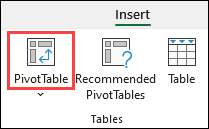
3. This will create a PivotTable based on an existing table or range.
   

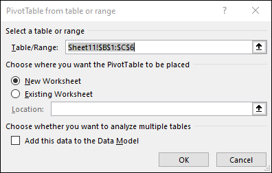
   Note: Selecting Add this data to the Data Model will add the table or range being used for this PivotTable into the workbook’s Data Model. Learn more.

4. Choose where you want the PivotTable report to be placed. Select New Worksheet to place the PivotTable in a new worksheet or Existing Worksheet and select where you want the new PivotTable to appear. 

5. Click OK